Project 2: Fun with Filters and Frequencies!
Part 1: Fun with Filters
1.1: Convolutions From Scratch!
For this part, I first started with a four for loop implementation that looped
through the entire padded image array. Then, for each ith, jth element in the
image array, we loop through the kernel, and get the sum of the element *
the kenel. We then set that as the ith, jth value of our output to get the
convoluted image.
This version took very very long, since it had to do single computation over every single pixel of the image.
For a 1500x2000 image, it took roughly 10 seconds to complete one convolution.
def brute_convolution_four(img_array, kernel):
    h, w = len(img_array), len(img_array[0])
    kh, kw = len(kernel), len(kernel[0])
    pad_h, pad_w = kh // 2, kw //2
    padded = np.pad(img_array, ((pad_h, pad_h), (pad_w, pad_w)), mode="constant")

    output = np.zeros_like(img_array, dtype=np.float64)
    for i in range(h):
        for j in range (w):
            total = 0
            for n in range(kh):
                for m in range(kw):
                    total += padded[i+n, j+m] * kernel[n, m]
            output[i, j] = total

    return output
I then made this faster using just two for loops, looping through the entire
padded image array, but taking a slice of the image array to do elementwise
multiplication of that slice with the kernel. After getting that product, I
summed it to get the final output and then set the ith, jth value as that sum.
This version was way faster, cutting down the computation time to around 2 seconds
to complete one convolution. It still wasn't close to the built in convolve2d, however,
since convolve2d was almost instantaneous.
def brute_convolution_two(img_array, kernel):
    h, w = len(img_array), len(img_array[0])
    kh, kw = len(kernel), len(kernel[0])
    pad_h, pad_w = kh // 2, kw //2
    padded = np.pad(img_array, ((pad_h, pad_h), (pad_w, pad_w)), mode="constant")
    output = np.zeros_like(img_array, dtype=np.float64)

    for i in range(h):
        for j in range(w):
            area = padded[i: i+kh, j:j+kw]
            output[i, j] = np.sum((area * kernel))
return output

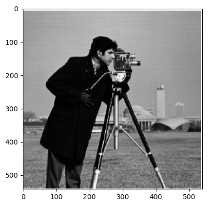
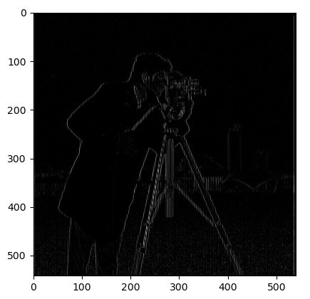
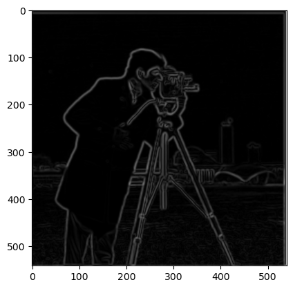
1.2: Finite Difference Operator
For this part, I used the built in scipy.convolve2d to convolve the cameraman image with the dy and dx filter. Then, I got the gradient by taking the euclidean distance between each value of the convoluted dy and dx images. I then tested different threshholds to figure out the best one to classify the edges. I tried 0.7 but it wasn't able to get some of the thinner ones, so I tried going down to 0.5, and then 0.3, then 0.1.
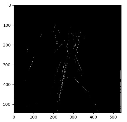
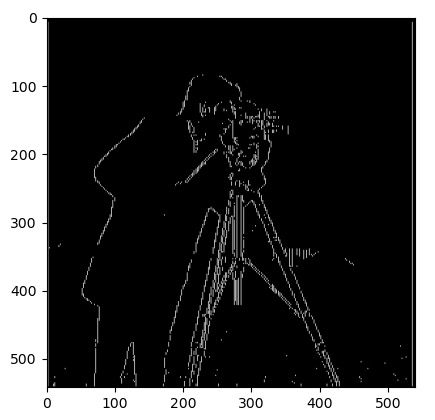
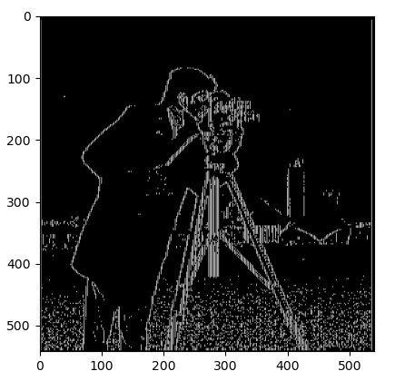
As I got to 0.3 and 0.1, a lot of noise started showing up. I couldn't get the real edges of the buildings in the back without the grass speckles using this method, so I decided to go back past 0.3 a little bit to reduce the noise as much as possible and just get the cameraman.
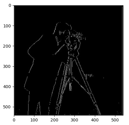
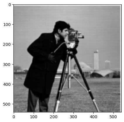
1.3: Derivative of Gaussian (DoG) Filter
For this part, I first created the 1D Guassian filter G using cv2.getGaussianKernel(). Then I created the 2D kernel by getting the outer product with it's transpose. Using that 2D kernel, I convolute the original image to smooth out the edges. I tried different inputs for the gaussian function, with 3 not smoothing well enough and 10 blurring the original image too much. I ended up with 6x1 as my sigma input to getGaussianKernel. After that, I just did the same dx, dy convolution on the smoothed image, and then got the gradient using np.hypot. After trialing a few thresholds, I ended up with a threshold of 0.12 now.

Now we try the single convolution by creating a derivative of gaussian filters. We first take the convolution of the gaussian filter with the dx and dy filters. Then we take the convolution of the cameraman image with these derived gaussian filters. Once we have those, we can get the gradient using np.hypot, and then filter the same threshhold to get the edge image.
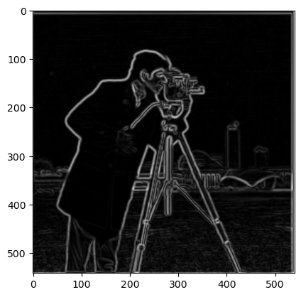
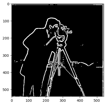
As we can tell, both the DoG filter and the original gaussian blurred edge image look the exact same.
Part 2: Fun with Frequencies!
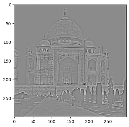
2.1: Image "Sharpening"
For this part, I first blurred the orignal grayscale image by convolving with a gaussian kernel, separating out the lower frequencies. Then, I got filtered out the lower frequencies by subtracting the greyscale image with the blurred grayscale image, getting only the high frequencies (the details). Then, I added the "details" back to the original image, using alpha = 0.8. Changing alpha changed how thick the lines from the details were and gave "more sharpening" as alpha increased and "less sharpening" as alpha decreased.
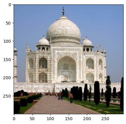
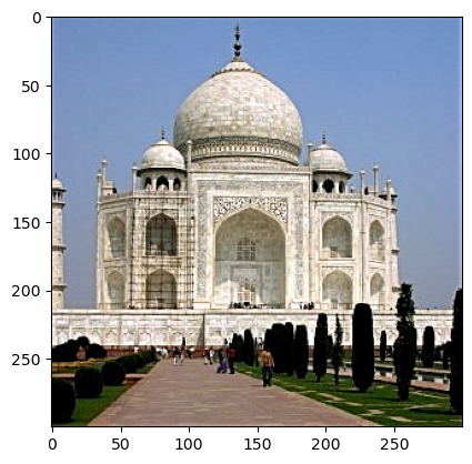
Taj Mahal:
The result was sharper edges on the Taj Mahal itself, with the tree silhouettes and streets emphasized, as we can see in the details image.
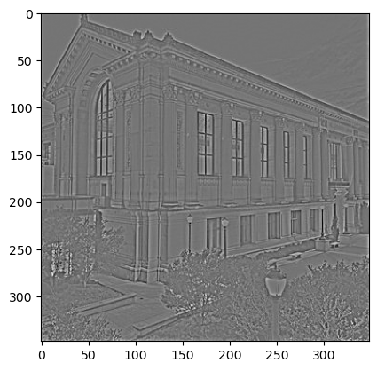
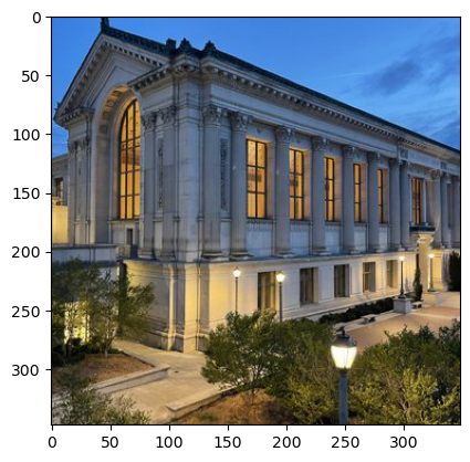
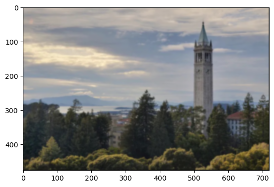
Doe Library:
For doe library, the building edges were also sharpened, and the tree details were enhanced. It almost looked like each branch was visible.

Blur and Resharpen:
For this, I first blurred an image with the original alpha = 10 gaussian kernel. Then, I did the same process to sharpen the image: gaussian blur the grayscale for the low frequencies, subtract those from the original grayscale to get the high frequencies, and then add it back to the original (blurred) color image.


The sharpening brought back some of the edges of the campanile, but was not able to unsmooth the edges of the trees or the smaller buildings in the back. A lot of the high frequencies were lost during our initial blurring, therefore even with the sharpening process, many of the edges could not be fully recovered.
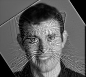
2.2: Hybrid Images
For this part, I did a high pass and low pass filter to filter out the high frequencies and low frequencies both images. For the low frequencies, I did a gaussian blur with kernel size = 6 * sigma1, and for the high frequenceies, I did a gaussian blur with kernel size 6 * sigma2, subtracting the original with the blur to get the high frequencies. I then added them together with a factor of alpha for the details to control how strong the high frequencies came out in the hybrid.
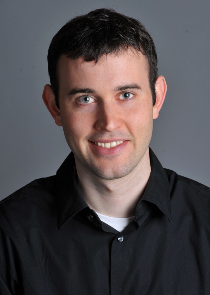
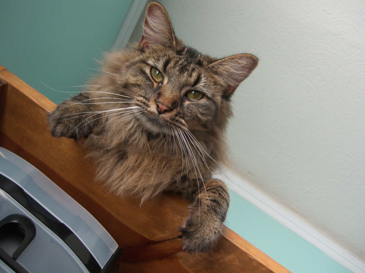
Derek + Nutmeg
Sigma1 = 3, Sigma2 = 5, alpha = 2. The edges of Nugmeg wasn't too prominent; I enhanced them so that Nutmeg was visible up close.
Messi + Ronaldo
Sigma1 = 3, Sigma2 = 5, alpha = 0.7. The edges of ronaldo came out very strong, so I lowered it so that Messi was still visible from afar.
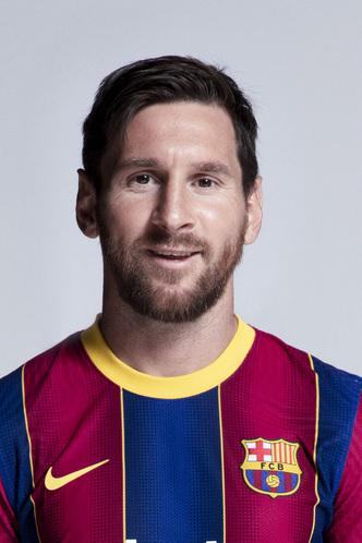
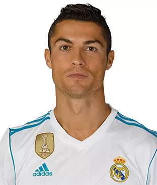
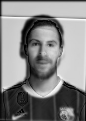
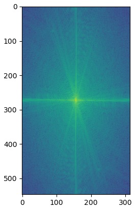
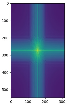
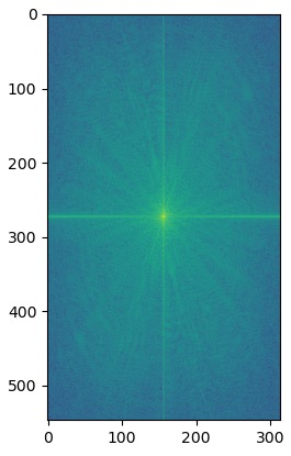
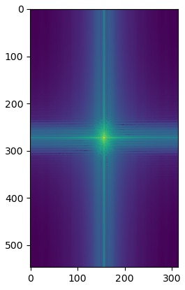
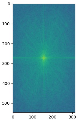
My favorite hybrid was Messnaldo, so I plotted the log magnitude of the Fourier transform for the images used to create it.
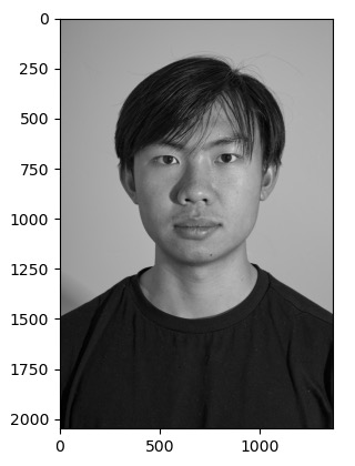
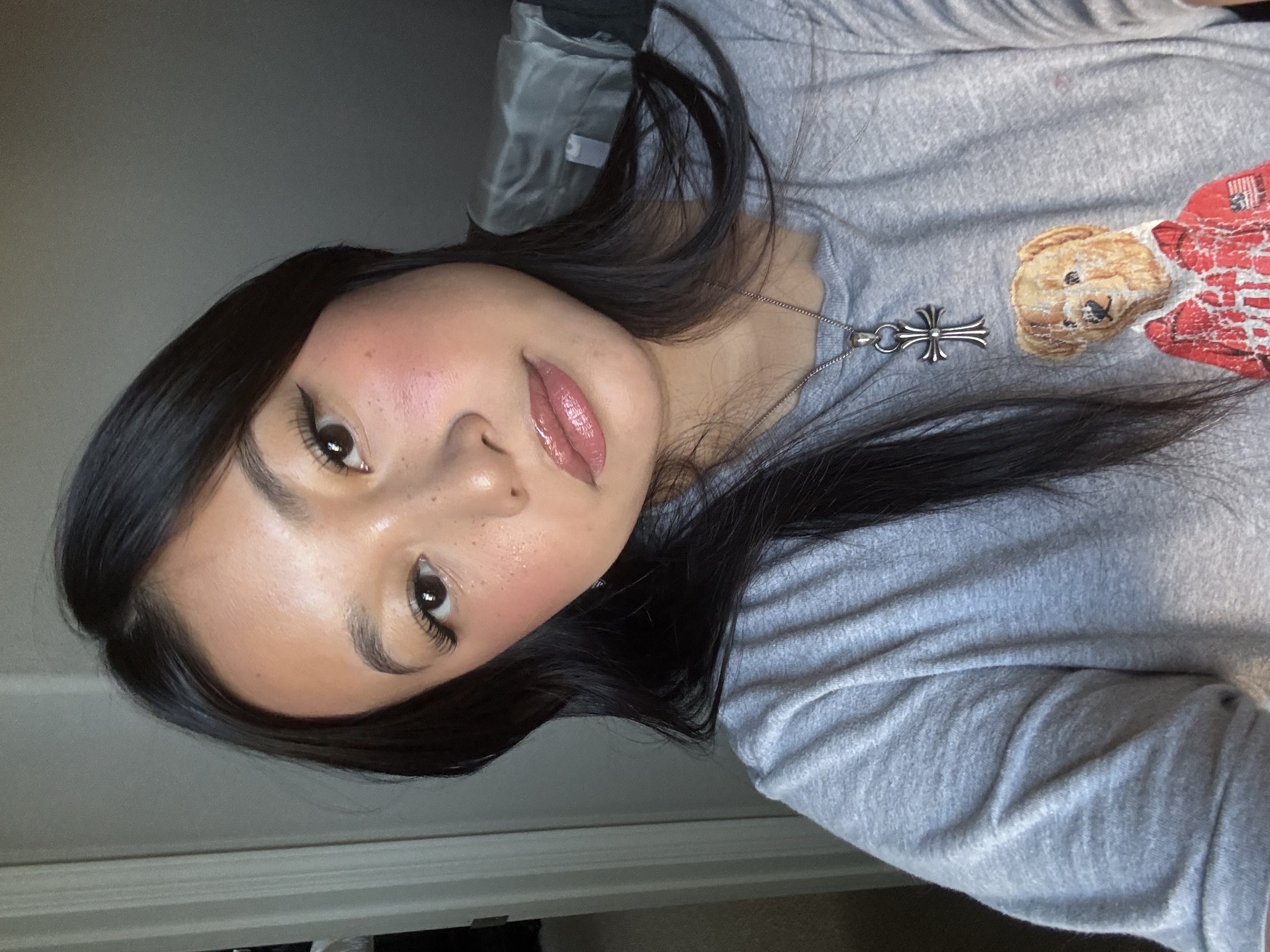
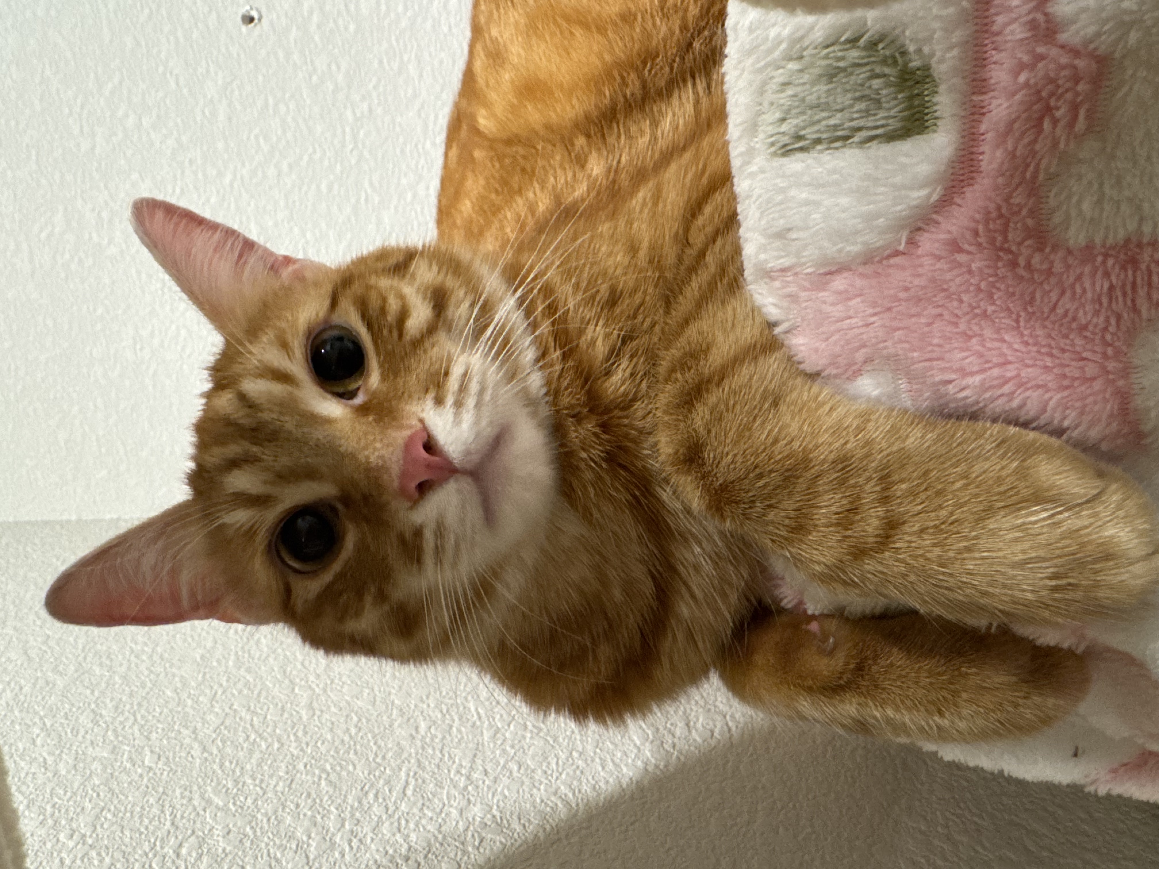
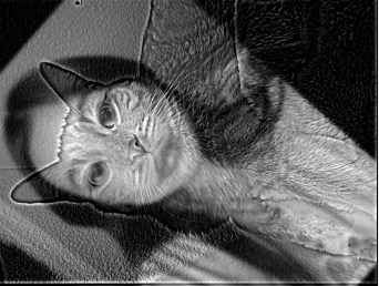
Jenn + Chicken the Cat
Sigma1 = 12, Sigma2 = 14, alpha = 2.5. The original images here were way bigger, so I had to do a bigger gaussian kernel to actually get a usable blur.
Multi-Resolution Blending and the Oraple Journey
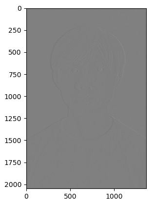
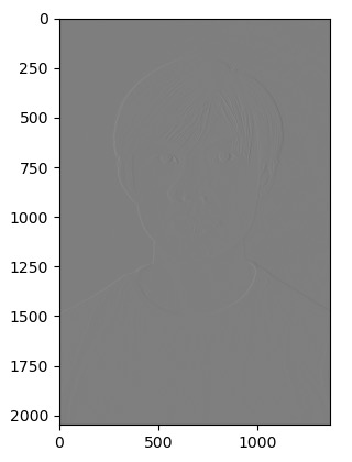
2.3: Gaussian and Laplacian Stacks
To build the Gaussian Stack, I repeatedly blurred the previous level with a noramalized gaussian kernal (6 * sigma) using reflect padding instead of fill padding. I didn't do any downsampling to keep the images the same size as the blur continued. To build the Laplacian stack, I took the differences between consecutive Gaussian levels - each Laplacian level was the current Gaussian level minus the next Gaussian level. As for the last Laplacian level, I just appeneded the last Gaussian level.
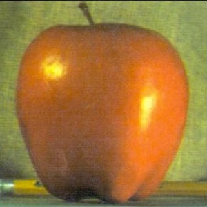
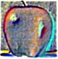
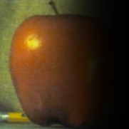
Apple Laplacian Stack (Levels 0-4)
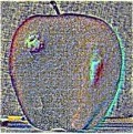
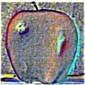
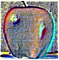
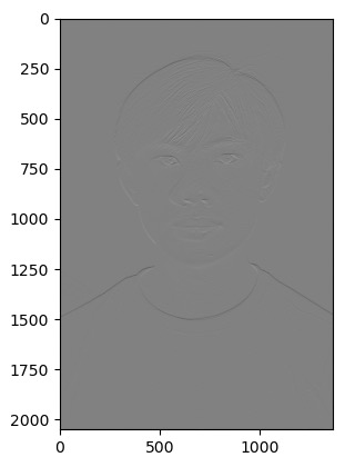
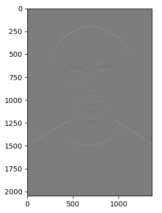
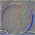
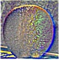
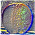
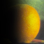
Orange Laplacian Stack (Levels 0-4)
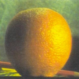
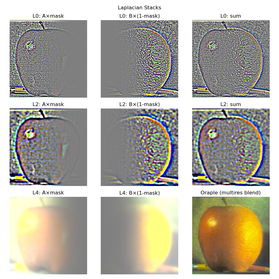
2.4: Multiresolution Blending (A.K.A. The Oraple!)
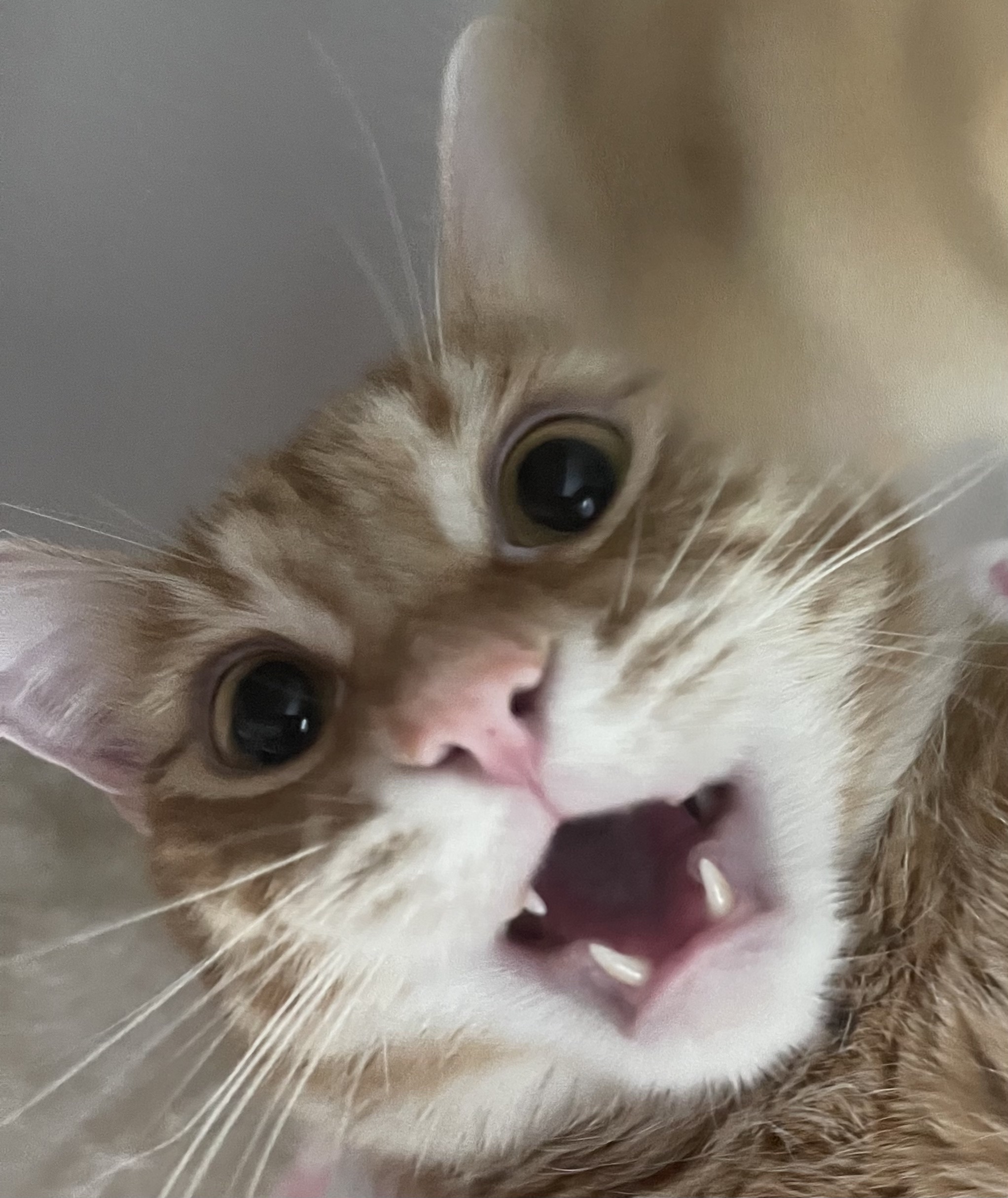
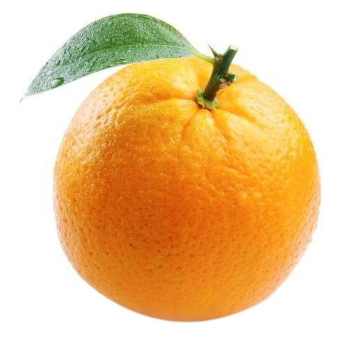
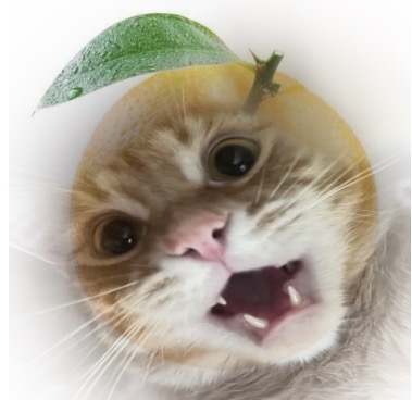
To actually blend images, I built the Laplacian stacks for both images with the same number of levels. Then, I generated a Gaussian stack from the mask input image. After that, I looped though each i, blending both Laplacian levels with the corresponding mask level. To get the final image, I sum over all the blended levels to get the correct pixel values. For my custom blend, I put a cat face onto an orange, using a circular mask to capture the cat's face.
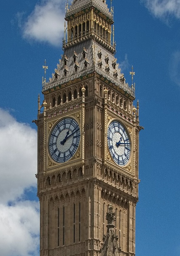
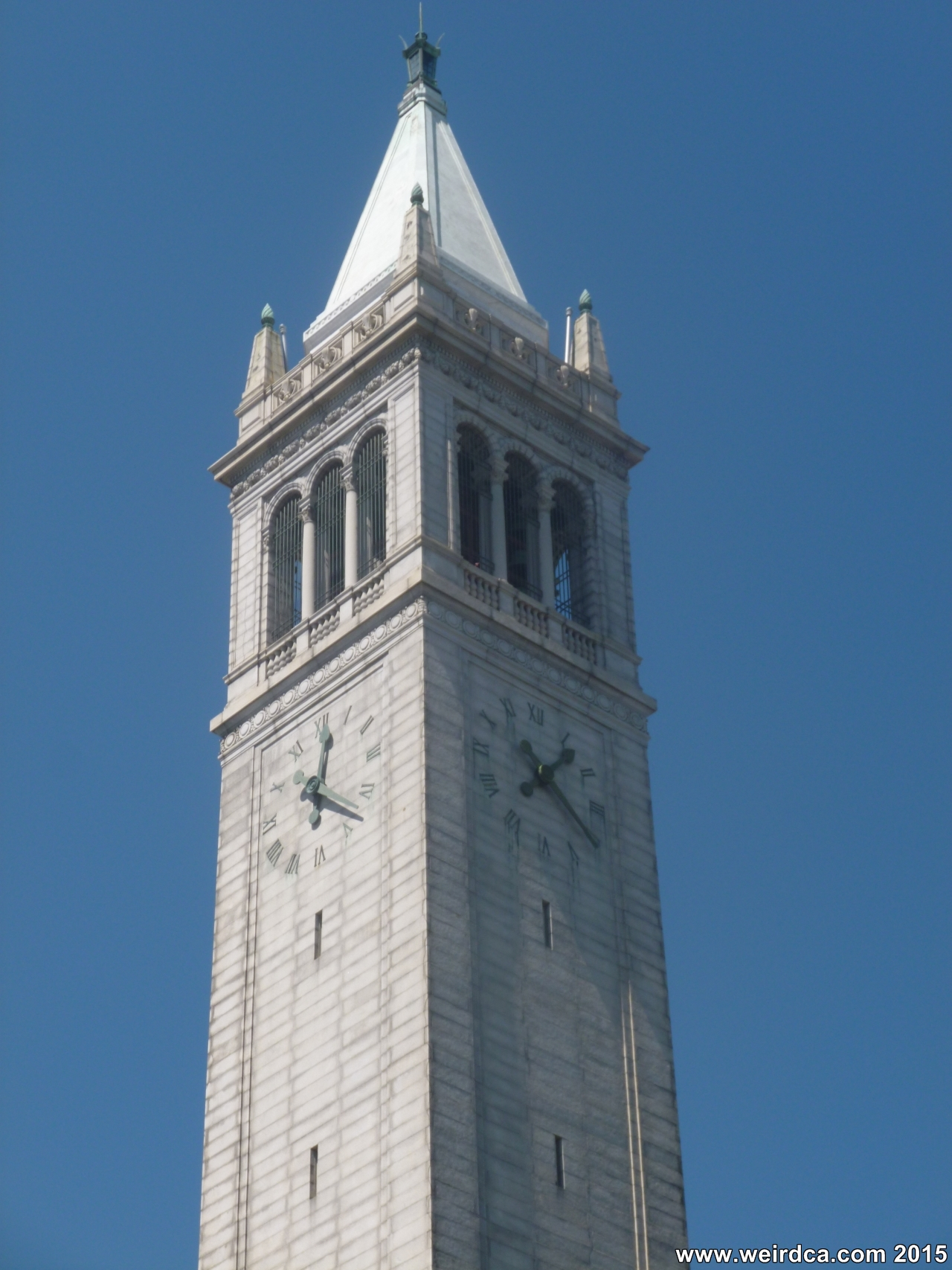
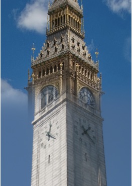
Campanile x Big Ben
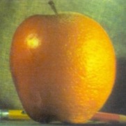
Chicken the Orange